Introduction

SDM is short for Supervised Descent Method. The original paper of SDM is published in CVPR 2013. Since then, I have explored several extensions of it, such as online SDM, global SDM. Also, I have spent some time on investigating its theoretical properties and applied it to other applications. The theoretical and experimental findings are submitted to TPAMI.

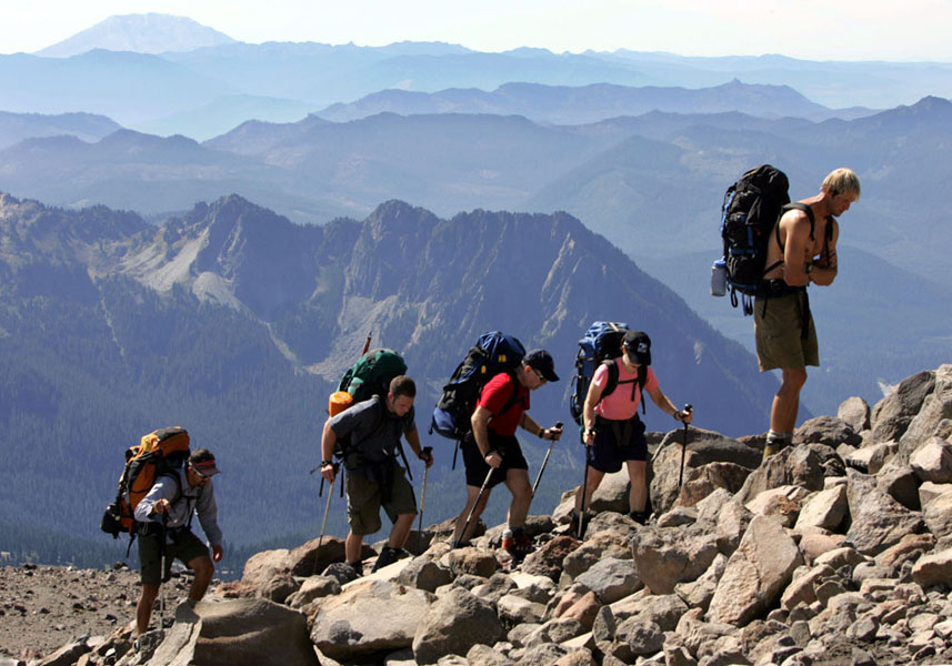
Originally, I developed SDM to optimize Nonlinear Least Squares (NLS) objectives. Here is a simple example illustrating how it differs from the traditional gradient-based methods. Optimization is like climbing a hill. Fig1. shows a "real-world" example of applying gradient-based methods to climb a hill. Alternatively, to reach the peak faster one can take a cable car (shown in Fig.2) although it takes the fun out of hiking. SDM proposes an offline procedure that builds the stationary ropes that carry the cable cars so in testing time the climb will be smooth and quick. Readers, please do not take it too literal, this example is supposed to only give you an intuition.

Descent Map I

Let us switch to the mathematical world. Say we want to minimize the following NLS function: $$ f(\x) = \min_\x \|\h(\x)-\y\|^2, $$ where $\x$ is the optimizing parameters, $\h$ is a nonlinear function, and $\y$ is a known vector. Below is the update equation from gradient-based methods: $$ \Delta x = \alpha\A\J^\top_\h(\x)(\h(\x)-\y), $$ where $\alpha$ is the step size, $\A$ is a rescaling factor, and $\J_\h$ is the Jacobian of $\h$ evaluated at the current parameter estimate $\x$. Different methods vary representation of $\A$. For example, $\A=\H^{-1}$ in Newton's method, $\A=(\J^\top\J)^{-1}$ in Gauss-Newton, $\A=\I$ in first-order methods. For non-differentiable functions, $\A$ and $\J$ are expensive to compute (e.g., one needs to use finite differences to approximate the Jacobian).

The main idea behind SDM is to replace this expensive term $\alpha\A\J_\h$ with a learned matrix $\R$. For now, you can think of $\R$ as the rope in the above example in Fig.2. In this paper, we formally defined $\R$ as Generic Descent Map (DM) and derived the conditions under which $\R$ can drive all samples to the global optimal solution.

SDM is an iterative algorithm that leans a sequence of DMs. Below, the animation shows a simple example of how SDM learns a sequence of DMs from the optimal trajectories (indicated by the dotted lines).

Descent Map II

Recently, I have found another interpretation of DM, thanks to Drew. If you are from a Robotics background, you may find this interpretation easier to understand. SDM tackles NLS problems from an Imitation Learning perspective by learning a sequence of optimization policies. Fig.4 shows the execution of descent policies learned following SDM.

Within this context, the state observation becomes this error $\h(\x)-\y$, the action corresponds to parameter update $\Delta\x$, and the DM can be seen as the policy that maps state observation to the action. The World is problem-specific and can be thought as the environment where you make your predictions. In many computer vision problems, the World is the input image so the environment is stationary.

Gradient-based methods can also be explained in the same framework. Recall that we use DM to replace this term, $\alpha\A\J_\h$ that can be seen as an optimization policy. However, this policy has to be derived online (e.g., the Jacobians need to be evaluated at the current parameter).